
[Paper Review] 2D Gaussian Splatting for Geometrically Accurate Radiance Fields
Introduction
In this post, I review 2D Gaussian Splatting for Geometrically Accurate Radiance Fields, a recent paper presented at CVPR 2024 by Binbin Huang et al. This work builds on the success of 3D Gaussian Splatting (3DGS) and introduces a novel approach for accurately modeling geometry and appearance using planar 2D Gaussian primitives embedded in 3D space. Unlike 3DGS, which struggles with thin surface reconstruction and multi-view consistency, 2D Gaussian Splatting (2DGS) addresses these limitations through a more surface-aligned formulation. This method enables high-fidelity geometry and photorealistic view synthesis from sparse input, making it a promising technique for applications such as novel view rendering, scene reconstruction, and AR/VR content creation.
Paper Info
- Title: 2D Gaussian Splatting for Geometrically Accurate Radiance Fields
- Authors: Binbin Huang, Zehao Yu, Anpei Chen, Andreas Geiger, Shenghua Gao
- Conference: SIGGRAPH 2024
- Paper: 2DGS
3D Gaussian Splatting Overview
To fully understand the improvements brought by 2D Gaussian Splatting, it’s helpful to understand the foundation laid by 3D Gaussian Splatting (3DGS). If you’re unfamiliar with 3DGS or want a refresher, check out my detailed technical review here:
👉 Understanding 3D Gaussian Splatting: A Technical Overview
In short, 3DGS represents scenes using volumetric 3D Gaussian primitives and renders them via differentiable splatting. While effective for view synthesis, it faces challenges with thin surface reconstruction, normal estimation, and multi-view consistency — all of which 2DGS aims to overcome.
2D Gaussian Splatting
To better reconstruct geometry while keeping the rendering photorealistic, this paper introduces 2D Gaussian Splatting (2DGS).
1. Modeling
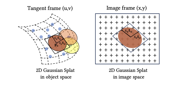
Compared to 3DGS, 2DGS simplifies things by using “flat” 2D Gaussians embedded in 3D space. Each splat lies in a local tangent plane and is defined by:
- A center point: pₖ
- Two tangential vectors: tᵤ, tᵥ
- A scaling vector: s = (sᵤ, sᵥ)
- A normal vector: t𝑤 = tᵤ × tᵥ
These form a rotation matrix:
\[R = [t_u, t_v, t_w]\]and a scaling matrix S, where the third row is zero. The transformation is defined as:
\[P(u, v) = p_k + s_u t_u u + s_v t_v v = H(u, v, 1, 1)^T\]with:
\[H = \begin{bmatrix} s_u t_u & s_v t_v & 0 & p_k \\ 0 & 0 & 0 & 1 \end{bmatrix}\]The 2D Gaussian value is:
\[G(u) = \exp\left(-\frac{u^2 + v^2}{2}\right)\]Each splat also carries an opacity α and a view-dependent color c, modeled with spherical harmonics.
2. Splatting
Affine Projection
Affine projection only works well at the center of the Gaussian and gets worse further out. To improve this, 2DGS uses homogeneous coordinates:
\[x = (xz, yz, z, z)^T = W H(u, v, 1, 1)^T\]To avoid numerical issues from matrix inversion, they apply:
\[h_u = (WH)^T h_x,\quad h_v = (WH)^T h_y\]Then solve for the intersection point by:
\[h_u \cdot (u, v, 1, 1)^T = h_v \cdot (u, v, 1, 1)^T = 0\]Which leads to:
\[u(x) = \frac{h_2^u h_4^v - h_4^u h_2^v}{h_1^u h_2^v - h_2^u h_1^v},\quad v(x) = \frac{h_1^u h_4^v - h_4^u h_1^v}{h_1^u h_2^v - h_2^u h_1^v}\]Degenerate Views
When a splat is viewed from the side, it can collapse into a line and be missed in rasterization. To avoid this, a low-pass filter is applied:
\[\hat{G}(x) = \max(G(u(x)), G(x - c, \sigma))\]with σ = √2 / 2, which ensures enough coverage even in edge cases.
Rasterization
Rasterization works like in 3DGS:
- Compute screen-space bounding boxes
- Sort Gaussians by depth
- Tile them into screen bins
- Apply volumetric alpha blending:
Training
Photometric loss alone isn’t enough — it often leads to noisy results. So two extra regularization losses are added.
1. Depth Distortion Loss
In 3DGS and its extensions, rendering is based on compositing semi-transparent Gaussian primitives, rather than directly modeling surface intersections. This can lead to geometry that is visually plausible in color but spatially imprecise — particularly when multiple splats along a ray contribute similar colors but differ in depth.
To resolve this, they introduce a depth distortion loss that encourages splats contributing to the same pixel to cluster tightly in depth. The formulation is:
\[L_d = \sum_{i,j} \omega_i \omega_j |z_i - z_j|\]- \(z_i\), \(z_j\): the depth values of splats i and j along a given ray.
- \(\omega_i\): the contribution (visibility) weight of splat i at that pixel, computed using alpha blending:
This encourages nearby splats to align along the viewing direction, reducing depth spread and sharpening the geometry. Unlike distortion terms used in prior methods (e.g., Mip-NeRF360), this version explicitly adjusts splat positions during training. The implementation uses optimized CUDA code for efficiency.
2. Normal Consistency Loss
Because each splat acts as a small surface patch, they also need to ensure their orientations match the underlying scene geometry. For this, they define a normal consistency loss:
\[L_n = \sum_i \omega_i (1 - n_i^\top N)\]- \(n_i\): normal vector of splat i, assumed to face toward the camera.
- \(N\): estimated surface normal at the pixel, derived from the local geometry.
- \(\omega_i\): visibility weight, as before.
To estimate the surface normal \(N\), they use finite differences of the rendered 3D position map \(p(x, y)\), computed from the splatted geometry:
\[N(x, y) = \frac{\nabla_x p \times \nabla_y p}{\|\nabla_x p \times \nabla_y p\|}\]This loss ensures the visible splats not only sit at the correct depth but are also oriented in a way that reflects the true surface — reducing shading artifacts and improving realism.
Final Loss
The model is trained using posed images and a sparse point cloud. The total loss is:
\[L = L_c + \alpha L_d + \beta L_n\]Where:
- L_c is the RGB reconstruction loss (L1 + D-SSIM)
- α = 1000 for bounded scenes, 100 for unbounded
- β = 0.05 across the board
Results
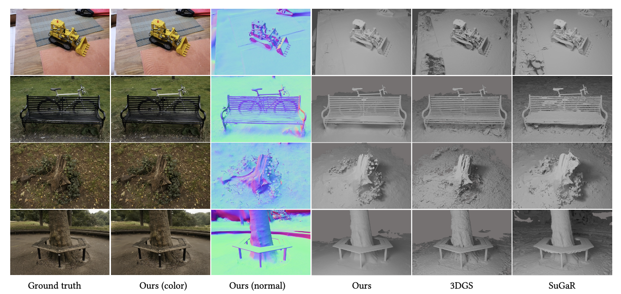
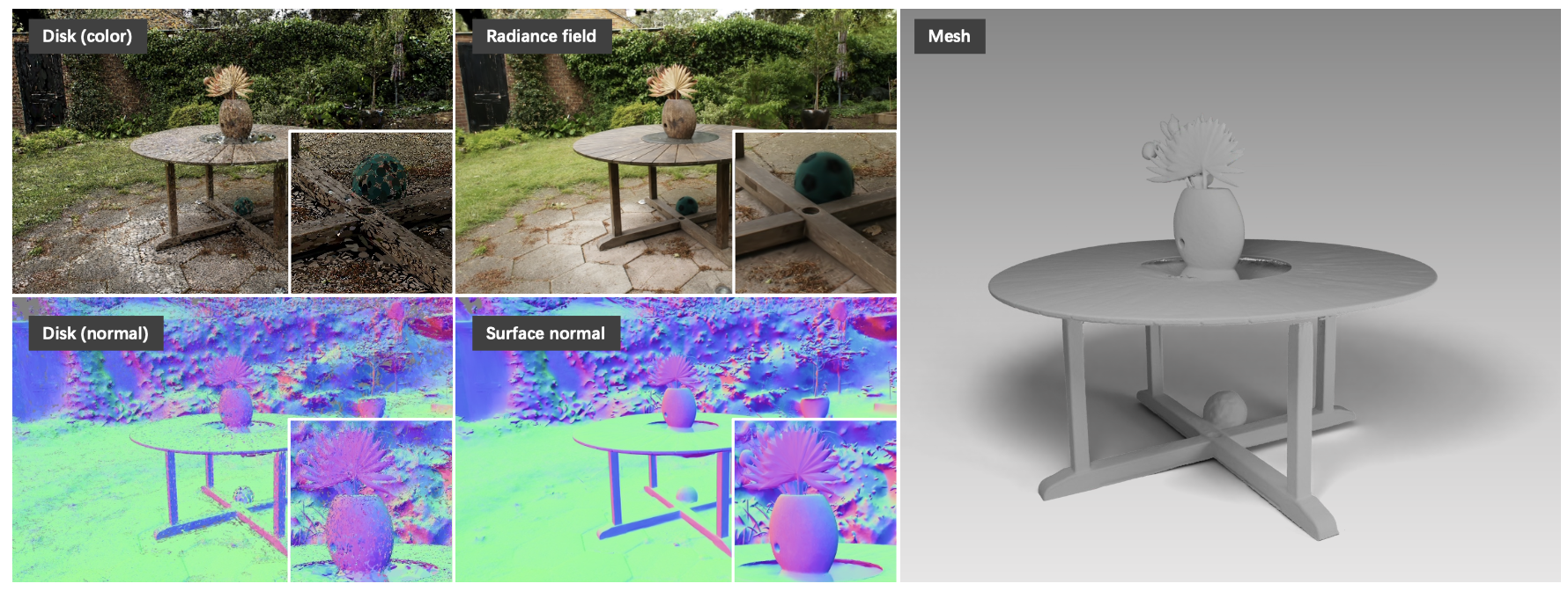
2D Gaussian Splatting delivers impressive results both in terms of geometry and novel view rendering. The qualitative comparisons show that 2DGS captures sharp edges, fine structures, and cleaner surfaces with fewer outliers, especially when reconstructing scenes like indoor objects or outdoor elements from the Mip-NeRF360 dataset. It’s also capable of producing high-quality novel view synthesis, competitive with top NeRF-based methods, but with the added benefit of accurate geometry.
What’s also cool is how efficiently it trains. On a single RTX 3090, it only takes around 5 to 18 minutes depending on the scene, and the final model is pretty lightweight (around 52MB in many cases).
Regularization also plays a big role — the depth distortion and normal consistency terms clearly improve surface sharpness and alignment. Ablation studies confirm that without them, the surfaces get noisy or misaligned.
As for mesh extraction, using TSDF fusion with median depth gives the cleanest results compared to expected depth or Poisson reconstruction, which can be more sensitive to outliers or ignore the opacity/scale info from Gaussians.
Limitations
While 2DGS performs really well in most cases, it’s not perfect.
- It assumes fully opaque surfaces, so things like glass or transparent materials aren’t handled well.
- Its current densification strategy favors areas with strong textures, meaning it might miss out on small geometric details in low-texture regions.
- There’s a trade-off between image quality and geometry sharpness during training — sometimes the regularization can cause oversmoothing in certain parts of the scene.
These are important to keep in mind if you’re applying 2DGS to scenes with complex material properties or trying to recover very fine details.