[Paper Review] 3D Gaussian Splatting for Real-Time Radiance Field Rendering

Introduction

This post provides a technical deep dive into “3D Gaussian Splatting for Real-Time Radiance Field Rendering”, a SIGGRAPH 2023 paper that shifts from implicit neural volume representations to explicit, differentiable rasterized primitives: anisotropic 3D Gaussians. It enables real-time photo-realistic rendering using standard GPU rasterization.

Paper Info

• Title: 3D Gaussian Splatting for Real-Time Radiance Field Rendering
• Authors: Bernhard Kerbl, Georgios Kopanas*, Thomas Leimkühler, George Drettakis
• Conference: SIGGRAPH 2023
• Paper: 3DGS PDF

Motivation and Context

Implicit radiance fields (e.g. NeRF) provide excellent results but suffer from poor interactivity, large inference times, and the need for neural network evaluations. This paper proposes:

• An explicit representation using 3D Gaussians
• A rasterization-based renderer with analytic derivatives
• High-speed optimization and rendering pipelines using standard graphics hardware

Scene Representation

Each point in the scene is modeled as a 3D anisotropic Gaussian parameterized by position, shape, opacity, and color. This allows for a compact and continuous representation of complex geometry.

Parameters of a 3D Gaussian:

\[F(x, v) \rightarrow (r, g, b, \alpha)\]

Where:

• Position:
  \(x \in \mathbb{R}^3\)
  The center (mean) of the 3D Gaussian in world space.

• Covariance Matrix:
  \(\Sigma \in \mathbb{R}^{3 \times 3}\)
  Describes the spatial extent and orientation of the Gaussian. It determines how the Gaussian “spreads” in 3D space.

  Specifically:

  • The eigenvalues of \(\Sigma\) control scaling along principal axes.
  • The eigenvectors (or rotation matrix from a quaternion) define the orientation of the ellipsoid.

  Implementation Note:
  In practice, \(\Sigma\) is not stored directly. Instead, it’s represented using:

  • A 3×1 vector of eigenvalues \(s = (s_1, s_2, s_3)\) (scale along each axis)
  • A quaternion or rotation matrix \(R\)
    Then:
    \(\Sigma = R \cdot \text{diag}(s^2) \cdot R^T\)

• Opacity:
  \(\alpha \in [0, 1]\)
  Controls the transparency of the Gaussian at that location. Used in alpha blending during volumetric rendering.

• Color:
  \((r, g, b)\) is not fixed, but varies based on the viewing direction \(v\). It is modeled using Spherical Harmonics (SH) to capture view-dependent appearance (e.g., specularities).

---

Color Computation with Spherical Harmonics

The RGB color of each Gaussian is a function of the viewing direction:

\[C(v) = \sum_{l=0}^L c^l Y^l(v)\]

Where:

• \(Y^l(v)\) are the spherical harmonic basis functions up to order \(L\) (typically 0–2 or 0–3).
• \(c^l \in \mathbb{R}^3\) are SH coefficients for each basis function and color channel.

This allows each Gaussian to express directional reflectance — such as how surfaces look brighter when facing the light or camera.

---

Rendering

Rendering is performed using volume rendering principles:

• Each Gaussian contributes a small amount of color and opacity to the final pixel along the ray.
• The color is accumulated using alpha compositing:

\[\text{final\_color} = \sum_i \alpha_i C_i(v) \prod_{j=1}^{i-1} (1 - \alpha_j)\]

Where each \(\alpha_i\) and \(C_i(v)\) come from a different Gaussian encountered along the ray.

This method produces smooth, view-dependent renderings of complex 3D scenes.

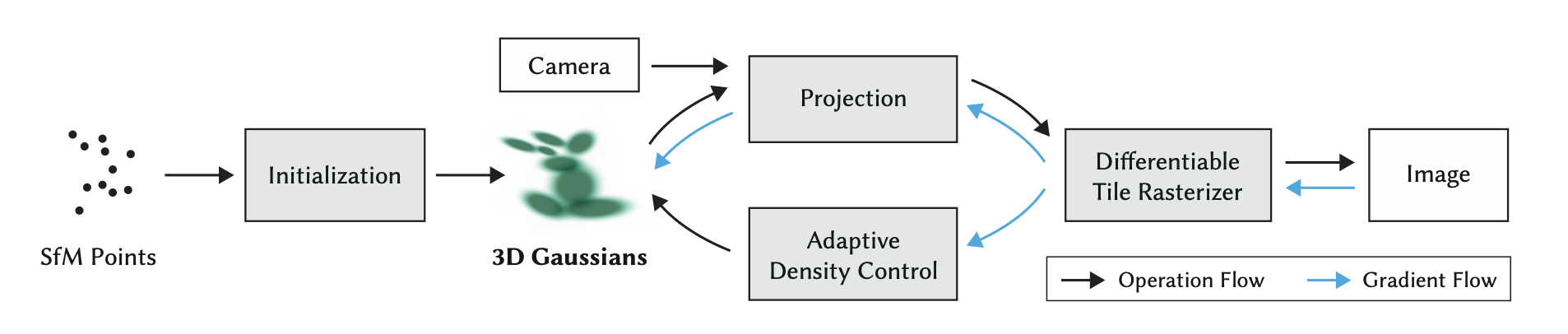
Rendering Pipeline

Gaussian Projection and Rasterization

Each Gaussian is projected into screen space as an ellipse using its 3D covariance. A resolution-adaptive quad is drawn using instanced rasterization with shader-based evaluation.

Per-tile Depth Sorting

Rendering uses alpha blending, which is not commutative. To handle this, the screen is divided into tiles, and Gaussians are sorted back-to-front within each tile before blending.

Visibility-aware Splatting

A visibility heuristic is applied to minimize overdraw. Gaussians far behind others or whose contributions are negligible are skipped.

Adaptive Density Control (ADC)

One key innovation is Adaptive Density Control, which actively regulates the number of Gaussians:

• Over-saturation: If a Gaussian consistently overlaps too many pixels or causes color saturation, it is split or shrunk. This is detected using the gradient norm and screen-space Jacobian.
• Under-coverage: Gaussians that fail to contribute significantly are merged or deleted. Low-density areas are up-sampled by duplicating and jittering existing Gaussians.
• Criteria include:
  • screen-space area
  • accumulated opacity
  • contribution to the loss gradient
  • overlap with neighbors (measured via elliptical coverage)

The algorithm monitors each Gaussian’s impact on the loss and its blending footprint, making it highly efficient and adaptive across scene complexity.

Training Procedure

Initialization

Training begins with a sparse point cloud reconstructed using COLMAP, which provides a 3D structure from multi-view images. Each point is initialized as a small isotropic Gaussian, with the initial covariance estimated as the mean distance to its three nearest neighbors. This gives a reasonable initial footprint for each Gaussian in 3D space.

Optimization Strategy

Training proceeds via iterative render-and-compare cycles. In each step:

• The current set of Gaussians is rendered to an image.
• The result is compared to ground truth views.
• Gradients are backpropagated to update Gaussian parameters.

Because projecting 3D geometry into 2D images is inherently ambiguous, the training must dynamically create, delete, and move Gaussians. This allows it to correct misalignments and converge toward a compact, accurate representation.

Optimization is performed using Stochastic Gradient Descent (SGD) within a GPU-accelerated framework. Critical steps like rasterization use custom CUDA kernels, enabling real-time training performance.

Activation Functions

To ensure valid parameter ranges and smooth gradients:

• Opacity \(\alpha\) is passed through a sigmoid to constrain it to \([0, 1)\).
• Covariance scaling is passed through an exponential function to maintain positive definiteness and stable optimization.

Loss Function

The loss is a weighted combination of L1 loss and D-SSIM (Differentiable Structural Similarity):

\[\mathcal{L} = (1 - \lambda) \cdot \mathcal{L}_{\text{L1}} + \lambda \cdot \mathcal{L}_{\text{D-SSIM}}\]

• L1 loss penalizes per-pixel absolute differences:

  \[\mathcal{L}_{\text{L1}} = \sum_{i} \left| I_i^{\text{rendered}} - I_i^{\text{GT}} \right|\]

• D-SSIM captures perceptual similarity by comparing local structures rather than raw pixel values. It is a differentiable variant of the SSIM metric, enabling effective supervision that preserves edges and textures.

The hyperparameter \(\lambda\) balances low-level accuracy and perceptual quality.

Learning Rate Schedule

A decaying learning rate is applied to the position updates, following the scheduling strategy used in Plenoxels. This improves stability and helps avoid overshooting as training progresses.

Differentiable Rasterization

The rendering process is fully differentiable. Each Gaussian is projected to an anisotropic 2D ellipse and blended in screen space. This projection and blending are implemented with efficient CUDA-based rasterization, which is the main computational bottleneck but remains fast enough for real-time training updates.

Regularization

• Covariance penalty prevents collapse
• Opacity clamping to keep gradients stable
• TV loss on SH coefficients for color smoothness

Evaluation

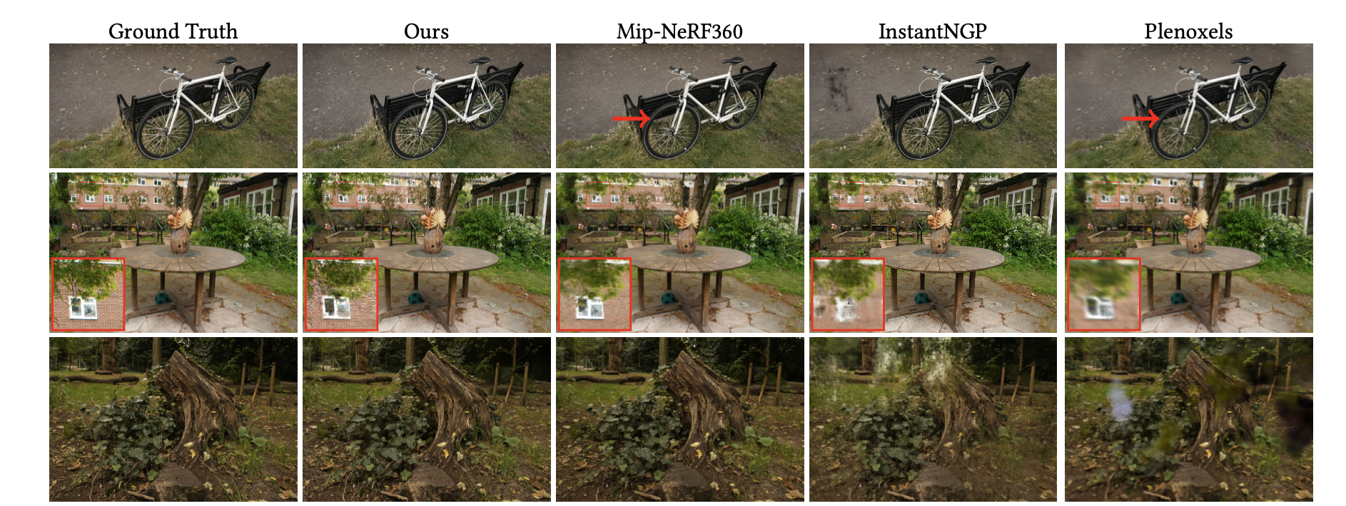
• Benchmarks on NeRF-Synthetic, Tanks and Temples, and Mip-NeRF 360 datasets
• Measured metrics: PSNR, SSIM, LPIPS
• Rendering FPS measured with screen resolution 800×800 on RTX 3090

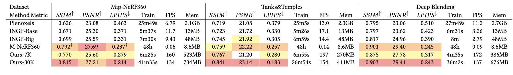
Results

Method	PSNR ↑	LPIPS ↓	FPS ↑	Training Time ↓
NeRF	31.0	0.15	<1	>10h
Instant-NGP	30.5	0.18	30–60	10–30 min
3D Gaussian Splatting	32.1	0.12	60–100	~30 min

Ablation Studies

• Anisotropy vs. Isotropy: removing anisotropy reduces detail
• No ADC: leads to overdraw, visual artifacts, GPU overload
• SH Order: higher orders model glossy materials better, but cost more
• Visibility Pruning: improves render time 3–5×

Limitations

• Static scenes only (no dynamic or relighting)
• Requires known camera poses
• Still slow for live capture due to COLMAP dependency
• Alpha blending may cause semi-transparency artifacts in dense regions

Conclusion

3D Gaussian Splatting offers a major breakthrough in real-time novel view synthesis by abandoning implicit neural fields in favor of explicit, interpretable, and efficient 3D primitives. It sets a new standard in speed vs. quality tradeoff and opens the door to real-time interaction in high-fidelity 3D vision.

Future directions include:

• Hybrid neural + Gaussian pipelines
• Dynamic scenes and time-dependent Gaussians
• Integration with neural textures or mesh structures

---

Next: A deep dive into Neural Splatting, an extension incorporating learnable splatting behaviors into this framework.