
[Paper Review] DUSt3R: Geometric 3D Vision Made Easy
Introduction
In this post, I perform a deep dive into DUSt3R: Geometric 3D Vision Made Easy, published at CVPR 2024 by Naver Labs Europe.
For the last two decades, the standard recipe for 3D reconstruction has been a rigid pipeline: Keypoints \(\to\)Matching\(\to\)Structure-from-Motion (SfM)\(\to\) Multi-View Stereo (MVS). This pipeline relies on explicit geometric constraints: if you don’t know your camera intrinsics, you must estimate them; if you can’t find sparse keypoints (e.g., on a white wall), the pipeline collapses.
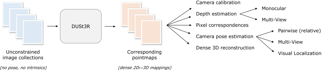
DUSt3R (Dense Unconstrained Stereo 3D Reconstruction) proposes a paradigm shift. It argues that we don’t need to explicitly solve for camera parameters or perform feature matching as a prerequisite. Instead, we can regress the dense 3D geometry directly from images using a powerful Transformer.
By relaxing the hard constraints of projective geometry, DUSt3R unifies Monocular Depth, Multi-View Stereo, and Pose Estimation into a single “Pointmap Regression” task.
Paper Info
- Title: DUSt3R: Geometric 3D Vision Made Easy
- Authors: Shuzhe Wang, Vincent Leroy, Yohann Cabon, Boris Chidlovskii, Jerome Revaud
- Affiliations: Naver Labs Europe
- Conference: CVPR 2024
- Project Page: DUSt3R GitHub
The Core Concept: The “Pointmap”
The fundamental innovation of DUSt3R is replacing the standard Depth Map with the Pointmap.
In traditional MVS, the output is a depth map \(D \in \mathbb{R}^{H \times W}\). A depth map is geometrically ambiguous without the camera intrinsics matrix \(K\). It describes distance along a ray, but doesn’t tell you where that ray is pointing.
A Pointmap \(X \in \mathbb{R}^{H \times W \times 3}\) contains the absolute 3D coordinate \((x,y,z)\) for every pixel \((u,v)\) in the image.
Implicit Calibration
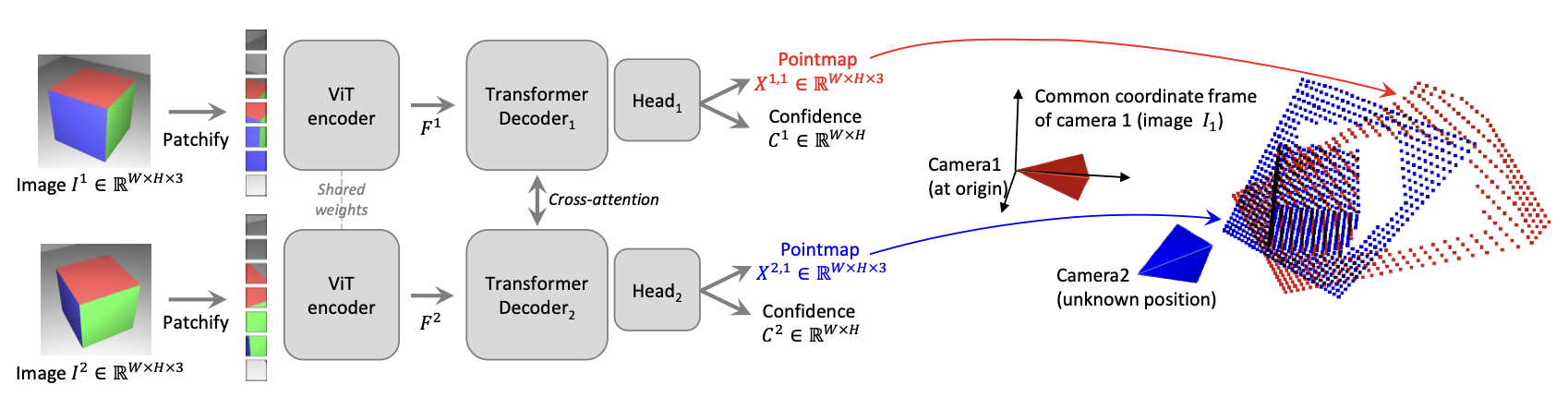
Critically, DUSt3R predicts these pointmaps in an unconstrained coordinate system. When fed a pair of images \(I_1\) and \(I_2\), it predicts two pointmaps \(X_{1,1}\) and \(X_{2,1}\):
- \(X_{1,1}\): The 3D geometry of View 1, expressed in View 1’s coordinate frame.
- \(X_{2,1}\): The 3D geometry of View 2, also expressed in View 1’s coordinate frame.
This is the “magic trick.” By forcing the network to predict View 2’s geometry in View 1’s frame, the network implicitly solves the relative pose \([R \mid t]\) between the cameras and applies it to the geometry. You don’t need to mathematically enforce epipolar constraints; the network learns them as a data-driven prior.
Methodology
1. Architecture: CroCo + Cross-Attention
The authors build upon CroCo (Cross-View Completion), a pre-training recipe for 3D vision. The architecture is a Siamese Vision Transformer (ViT):
- Siamese Encoder: Both images share the same weights. They are tokenized into patches (\(16 \times 16\)).
- Cross-Attention Decoder: This replaces the “Matching” step of traditional pipelines. The decoder blocks alternate between Self-Attention (understanding the context within one image) and Cross-Attention (querying the other image).
- Intuition: When the network processes a pixel of a “corner” in Image 1, the Cross-Attention mechanism looks at Image 2 to find the corresponding “corner.” This provides the geometric cues needed to triangulate the depth.
- Prediction Heads: The network outputs:
- Pointmaps: \(X \in \mathbb{R}^{H \times W \times 3}\)
- Confidence Maps: \(C \in \mathbb{R}^{H \times W}\). This tells us which pixels are valid (e.g., rigid objects) and which are invalid (e.g., sky, dynamic objects, lens flares).
2. Training Objective
The loss function is surprisingly simple. It is a direct regression loss in 3D space, weighted by confidence:
\[\mathcal{L} = \sum_{v \in \{1,2\}} \sum_{i \in \text{valid}} C_{v,i} \left\| X_{v,i} - \frac{1}{z} \bar{X}_{v,i} \right\| - \alpha \log C_{v,i}\]- Regression Term: Minimizes the Euclidean distance between predicted point \(X\) and ground truth \(\bar{X}\).
- Scale Normalization (\(z\)): Since the scene scale is ambiguous from images alone, both prediction and ground truth are normalized by their average depth.
- Confidence Regularizer (\(-\alpha \log C\)): Prevents the network from “cheating” by predicting zero confidence everywhere. It forces the network to assign high confidence to pixels where the geometric error is low.
From Pairs to Scenes: Global Alignment
The network described above only works on pairs of images. Real-world reconstruction involves dozens or hundreds of images. How do we fuse them?
Traditional pipelines use Bundle Adjustment, which minimizes 2D Reprojection Error (\(\sum \|u - \pi(PX)\|^2\)). This is non-convex and sensitive to initialization.
DUSt3R introduces Global Alignment. It constructs a “Connectivity Graph” where images are nodes and pairs are edges. Since every edge (pair) provides a partial 3D reconstruction (\(X_{n,e}\) and \(X_{m,e}\)), we simply need to align these 3D point clouds rigidly.
The optimization objective minimizes 3D Projection Error:
\[\chi^*, P^* = \text{argmin}_{\chi, P, \sigma} \sum_{e \in E} \sum_{v \in e} \| \chi_v - \sigma_e P_e X_{v,e} \|^2\]- \(\chi_v\): The final, global pointmap for view \(v\).
- \(P_e\): The absolute pose of the camera.
- \(\sigma_e\): A scaling factor (to handle the scale ambiguity of each pair).
- \(X_{v,e}\): The raw pairwise prediction from the network.
Why is this better? Aligning 3D point clouds is a much easier optimization problem than Bundle Adjustment. It converges faster and is far less likely to get stuck in local minima.
DUSt3R as a “Swiss Army Knife”
Because the Pointmap encodes so much information, DUSt3R can effectively perform almost any 3D task by post-processing the output:
1. Relative Pose Estimation
You want the pose matrix \(T_{1\to2}\)? Simply take the two predicted point clouds \(X_{1,1}\) and \(X_{2,1}\). Since \(X_{2,1}\)is essentially\(X_{2,2}\) transformed into View 1, you can recover the transformation using Procrustes Alignment (Singular Value Decomposition).
2. Intrinsic Estimation
You want the focal length \(f\)? Since \(X_{i,j} = (x,y,z)\) corresponds to pixel \((u,v)\), and we know \(u = f \frac{x}{z} + c_x\), we can solve for \(f\) using a simple least-squares optimization on the predicted pointmap.
3. Pixel Matching
You want to find where pixel \(p_1\) in Image 1 is in Image 2?
- Look up the 3D coordinate of \(p_1\) in \(X_{1,1}\).
- Search for the closest 3D point in \(X_{2,1}\) (Nearest Neighbor search).
- The pixel associated with that point is your match. This allows for dense, sub-pixel matching without ever computing descriptors.
Results & Versatility
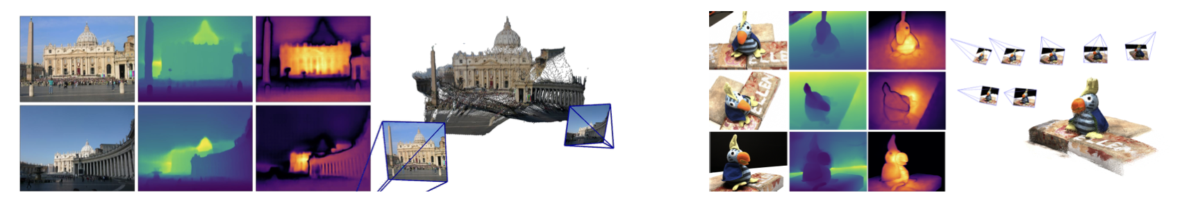
Performance Highlights:
- Map-free Localization: DUSt3R achieves state-of-the-art results (0.98m median error), significantly beating feature-matching pipelines like LoFTR + RANSAC.
- Multi-View Stereo: On the DTU dataset, it performs competitively with methods that require ground-truth poses, despite DUSt3R using none.
- Monocular Depth: By feeding \((I, I)\) into the network, it functions as a state-of-the-art monocular depth estimator.
Critical Analysis
Strengths
- Robustness to “Junk” Data: DUSt3R works on textureless walls, repetitive patterns, and wide baselines where SIFT/SuperGlue fail. The global context of the Transformer solves ambiguities that local features cannot.
- Simplicity: It removes the need for tuning hyperparameters in RANSAC, Essential Matrix estimation, or patch match stereo.
Limitations
- Computational Cost (\(O(N^2)\)): The Global Alignment requires running the network on pairs of images. For a sequence of \(N\) images, naively running all pairs is expensive. (This is exactly what Spann3R solves by making the process sequential/linear).
- Metric Scale: Like all monocular/stereo learning methods, it cannot recover true metric scale (meters) without external priors or sensor data.
- Memory Hog: Storing dense pointmaps (\(H \times W \times 3 \times \text{Float32}\)) for every pair in a large graph consumes significant VRAM and RAM compared to sparse features.
Takeaways
DUSt3R is a glimpse into the future of 3D Computer Vision. It suggests that the decades-old separation of “Calibration” and “Reconstruction” is artificial. By letting a Transformer learn the geometry end-to-end, we get a system that is:
- Robust: Works on textureless surfaces where COLMAP fails.
- Simple: No need to tune RANSAC thresholds or matching heuristics.
- Unified: One model for Monocular, Stereo, and MVS tasks.
For researchers, this paper opens the door to “Geometry as Regression”, moving away from “Geometry as Optimization.”